Датотека:Aliasing between a positive and a negative frequency.png
Већа резолуција није доступна.
Aliasing_between_a_positive_and_a_negative_frequency.png (694 × 452 пиксела, величина датотеке: 44 kB, MIME тип: image/png)
| Ово је датотека са Викимедијине оставе. Информације са њене странице са описом приказане су испод. Викимедијина остава је складиште слободно лиценциралних мултимедијалних датотека. И Ви можете да помогнете. |
Опис измене
| Опис |
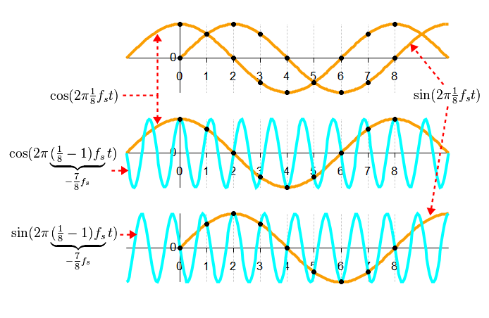
English: This figure depicts two complex sinusoids, colored gold and cyan, that fit the same sets of real and imaginary sample points. They are thus aliases of each other when sampled at the rate (fs) indicated by the grid lines. The gold-colored function depicts a positive frequency, because its real part (the cos function) leads its imaginary part by 1/4 of one cycle. The cyan function depicts a negative frequency, because its real part lags the imaginary part. |
|||
| Датум | ||||
| Извор | Сопствено дело | |||
| Аутор | Bob K | |||
| Дозвола (Поновно коришћење ове датотеке) |
Ја, носилац ауторског права над овим делом, објављујем исто под следећом лиценцом:
|
|||
| Остале верзије |
Derivative works of this file: Aliasing between a positive and a negative frequency.svg
|
|||
| PNG genesis | This PNG graphic was created with LibreOffice. |
|||
| Octave/gnuplot source | click to expand
This graphic was created with the help of the following Octave script: graphics_toolkit gnuplot
gold = [251 159 3]/256; % arbitrary color choice
sam_per_sec = 1;
T = 1/sam_per_sec; % sample interval
dt = T/20; % time-resolution of continuous functions
cycle_per_sec = sam_per_sec/8; % sam_per_sec = 8 * cycle_per_sec (satisfies Nyquist)
figure
subplot(3,1,1)
xlim([-2 10])
ylim([-1.3 1.3])
% Plot cosine function
start_time_sec = -2;
stop_time_sec = 10;
x = start_time_sec : dt : stop_time_sec;
y = cos(2*pi*cycle_per_sec*x);
plot(x, y, "color", gold, "linewidth", 4)
box off % no border around plot please
hold on % same axes for next 3 plots
% Plot sine function
start_time_sec = 0;
stop_time_sec = 10;
x = start_time_sec : dt : stop_time_sec;
y = sin(2*pi*cycle_per_sec*x);
plot(x, y, "color", gold, "linewidth", 4)
% Sample cosine function at sample-rate (1/T)
start_time_sec = 0;
stop_time_sec = 8;
x = start_time_sec : T : stop_time_sec;
y = cos(2*pi*cycle_per_sec*x);
plot(x, y, "color", "black", ".")
% Sample sine function
y = sin(2*pi*cycle_per_sec*x);
plot(x, y, "color", "black", ".")
set(gca, "xaxislocation", "origin")
set(gca, "yaxislocation", "origin")
set(gca, "xgrid", "on");
set(gca, "ygrid", "off");
set(gca, "ytick", [0]);
set(gca, "xtick", [0:8]);
subplot(3,1,2)
xlim([-2 10])
ylim([-1.3 1.3])
cycle_per_sec2 = cycle_per_sec - sam_per_sec; % negative frequency
% Re-plot same cosine function on new axes
start_time_sec = -2;
stop_time_sec = 10;
x = start_time_sec : dt : stop_time_sec;
y = cos(2*pi*cycle_per_sec*x);
plot(x, y, "color", gold, "linewidth", 4)
box off
hold on
% Plot other cosine function
start_time_sec = -2;
stop_time_sec = 10;
x = start_time_sec : dt : stop_time_sec;
y = cos(2*pi*cycle_per_sec2*x);
plot(x, y, "color", "cyan", "linewidth", 4)
% Sample cosine functions at sample-rate (1/T)
start_time_sec = 0;
stop_time_sec = 8;
x = start_time_sec : T : stop_time_sec;
y = cos(2*pi*cycle_per_sec*x);
plot(x, y, "color", "black", ".")
set(gca, "xaxislocation", "origin")
set(gca, "yaxislocation", "origin")
set(gca, "xgrid", "on");
set(gca, "ygrid", "off");
set(gca, "ytick", [0]);
set(gca, "xtick", [0:8]);
subplot(3,1,3)
xlim([-2 10])
ylim([-1.3 1.3])
% Re-plot original sine function on new axes
start_time_sec = 0;
stop_time_sec = 10;
x = start_time_sec : dt : stop_time_sec;
y = sin(2*pi*cycle_per_sec*x);
plot(x, y, "color", gold, "linewidth", 4)
box off
hold on
% Plot other sine function
start_time_sec = -2;
stop_time_sec = 10;
x = start_time_sec : dt : stop_time_sec;
y = sin(2*pi*cycle_per_sec2*x);
plot(x, y, "color", "cyan", "linewidth", 4)
% Sample sine functions at sample-rate (1/T)
start_time_sec = 0;
stop_time_sec = 8;
x = start_time_sec : T : stop_time_sec;
y = sin(2*pi*cycle_per_sec*x);
plot(x, y, "color", "black", ".")
set(gca, "xaxislocation", "origin")
set(gca, "yaxislocation", "origin")
set(gca, "xgrid", "on");
set(gca, "ygrid", "off");
set(gca, "ytick", [0]);
set(gca, "xtick", [0:8]);
|


Историја датотеке
Кликните на датум/време да бисте видели тадашњу верзију датотеке.
| Датум/време | Минијатура | Димензије | Корисник | Коментар | |
|---|---|---|---|---|---|
| тренутна | 07:26, 27. март 2013. | | 694 × 452 (44 kB) | Bob K | User created page with UploadWizard |
Употреба датотеке
Следећа страница користи ову датотеку:
Глобална употреба датотеке
Други викији који користе ову датотеку:
- Употреба на ms.wikipedia.org